
Quantifying Luck - Any Monkey Can Beat The Market
How much does luck influence stock market returns?

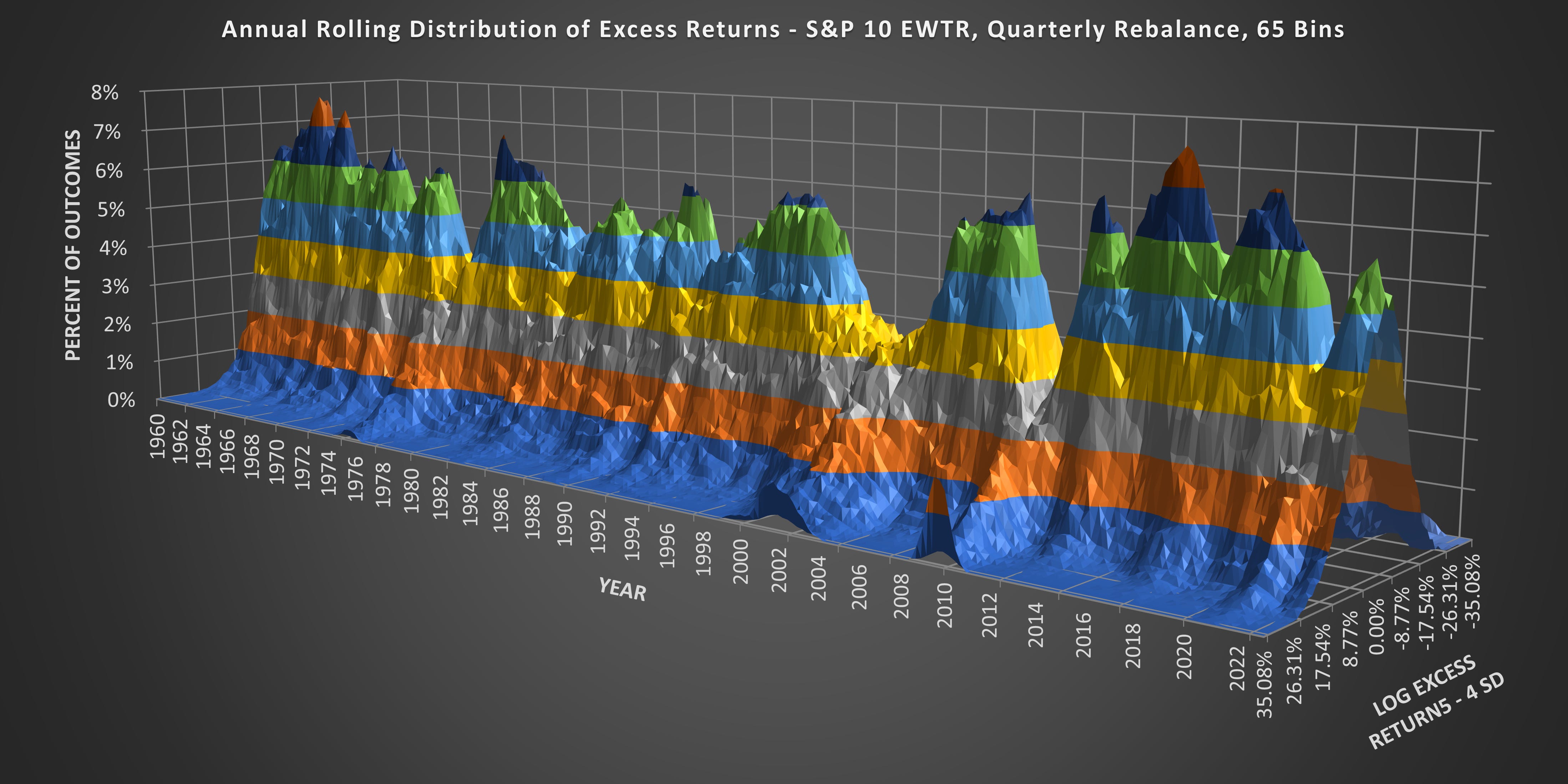
I suspect that many people will drop out before reading far through this article, so let’s start with a beautiful chart. Creating it required over 62 billion calculations and took weeks of work. If nothing else then hopefully you will enjoy the beauty. We will revisit this chart later on.
In his bestselling book, ‘A Random Walk Down Wall Street’, Burton Malkiel famously claimed that; “A blindfolded monkey throwing darts at a newspaper's financial pages could select a portfolio that would do just as well as one carefully selected by experts.”
Robert Arnott and the team from Research Affiliates LLC put this claim to the test and found that the Monkeys were able to beat the market 96 times out of 100!
Wait… WHAT? How is that possible?

It turns out that the benchmark we, as an industry, use - the S&P 500 - is a poor choice. Indices weighted by market cap disproportionately favor larger companies, increasing their holdings as prices rise while reducing their holdings in smaller companies. Outperforming the S&P 500 is as simple as selecting stocks based on ANY factor that avoids overweighting large companies. (Even if that 'factor' involves a monkey throwing darts!)
Eugene Fama and Kenneth French developed a five-factor model that enhances the explanation of portfolio returns by accounting for several dimensions of risk. The factors include:
Market Risk: Often quantified as the excess return of a portfolio over the risk-free rate, but more accurately; the sensitivity of a stock or portfolio to the overall market's excess return over the risk-free rate (represented by the market beta).
Size: Small-cap stocks tend to have higher returns than large-cap stocks, as measured by market capitalization.
Value: High book-to-market stocks tend to yield higher returns compared to low book-to-market stocks. This is often interpreted as a sign that "value" stocks are undervalued by the market.
Profitability: Companies with higher profitability, typically measured by earnings before interest and taxes (EBIT) divided by book value of equity, tend to outperform those with lower profitability.
Investment: Firms with low investment rates (conservative asset growth) tend to outperform firms with high rates of investment. This is typically measured by the change in total assets of the firm.
Additionally, while not part of the Fama-French model, two other popular factors include:
Momentum: This factor captures the tendency of stocks that have performed well in the past to continue performing well in the near future.
Volatility: This strategy involves selecting stocks with historically lower price fluctuations, aiming to reduce portfolio risk and potentially deliver more stable returns.
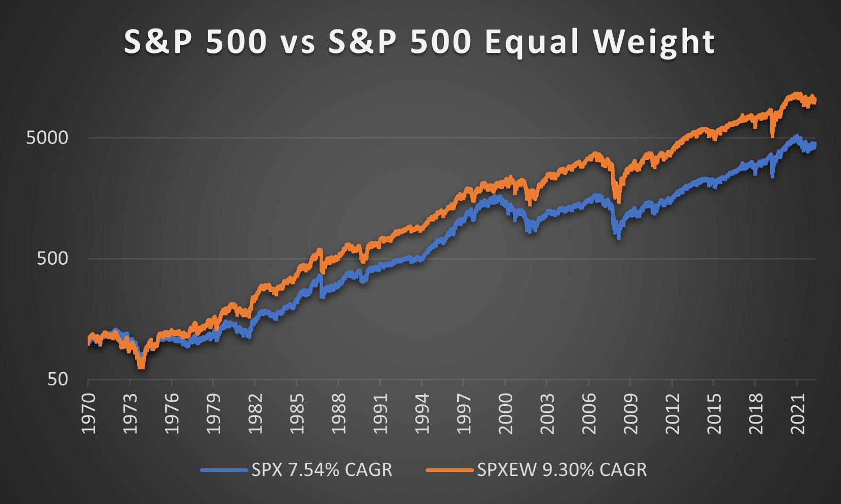
The S&P 500 Equal Weight Index (SPXEW) has achieved a Compound Annual Growth Rate (CAGR) of 9.3% since its inception in 1971, compared to 7.45% for the traditional S&P 500 over the same period. This resulted in 1.76% greater yearly returns simply by avoiding over-concentration in large companies.
So why is the S&P 500 the benchmark? Because a market cap-weighted index fund can absorb the most capital, meaning more fees for Wall St.
Most active managers who outperform the S&P 500 are simply benefiting from a factor slant, which may not even be intentional. Nevertheless, they attribute any outperformance to skill and charge a handsome fee for their genius!
If monkeys beat the market then I have questions…
1 - How much of a portfolio’s annual performance can be attributed to good or bad luck?
2 - How do the number of stocks in a portfolio and the rebalance frequency impact the range of possible outcomes and the sharp ratio?
To answer these questions I constructed a series of portfolios selected at random from the holdings of the S&P 500.
(Parameters and a glossary of terms have been included at the end of this article.)
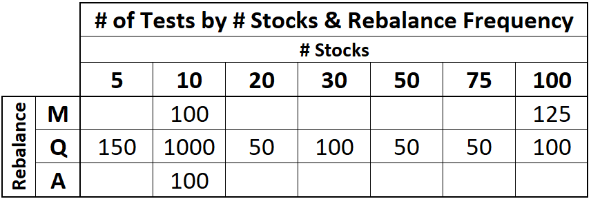
(Above) I simulated 1825 random portfolios and the table shows how many simulations were run for each portfolio size (# Stocks) and rebalance frequency. The richest data was gathered on portfolios with 10 stocks, rebalanced quarterly. 1000 tests were conducted in this range and are annotated as “S&P 10 EWTR” or “SPXEW 10” on the charts through this article. Unless otherwise stated the rebalance requence frequency is quarterly and the full 1957 - 2023 range has been used.
Distribution of Outcomes
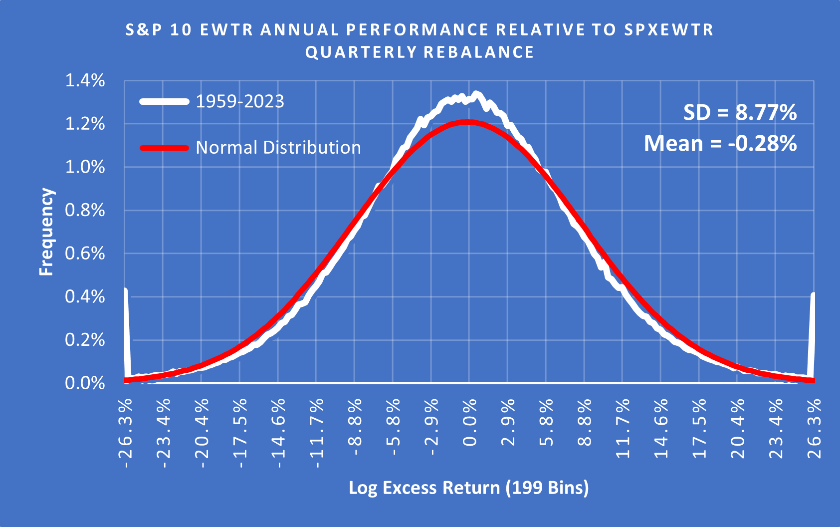
(Above) This is the probability distribution of excess returns for the S&P 10 EWTR rebalanced quarterly, 1957 - 2023. The Standard Deviation (SD) of 8.77% means that in a normal distribution, roughly 68.2% of the time, through pure luck you can expect outcomes +/- 8.77% relative to the benchmark in any given year. The X-Axis covers 3 SD.
However, the probability distribution curve isn’t normally distributed; it is Leptokurtic. While it looks normal-ish, it has a higher peak and fatter tails. In this instance, 0.82% of the annual outcomes were +/- more than 26.3% relative to the benchmark or > 3 Standard Deviations (3σ Sigma) from the mean. When people talk about tail risk they are referring to the over-representation of these extreme outcomes.
1 in 122 fund managers can be expected to either get very lucky or unlucky each year with a result +/- 3 SD. If the stock market was normally distributed then only 1 in 33,333 would land more than 3 SD from the mean purely through luck.
In a normal distribution you can expect outcomes relative to the mean:
68.27% <= 1 SD
27.18% > 1 SD <= 2 SD
4.55% > 2 SD
Over 20 years, you can expect portfolio performance outcomes relative to the benchmark to appear somewhat normally distributed. But from year to year the outcomes will be anything but normal.
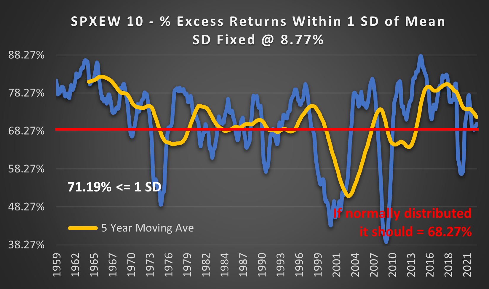
(Above) Using a constant SD @ 8.77 (the SD for the entire period 1959 - 2023), over the long term, the outcomes within 1 SD are only slightly more peaked than a Normal Distribution @ 71.19%. But the range from year to year is 38 - 88%. This makes financial markets notoriously difficult to model.
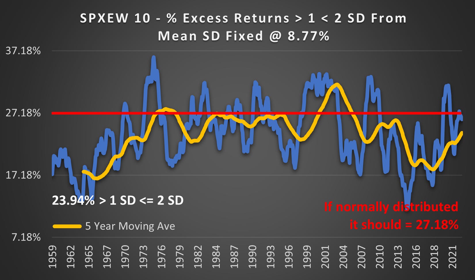
(Above) The 1 - 2 SD range is the most underrepresented @ 23.94%. It should be 27.18% in a normal distribution.
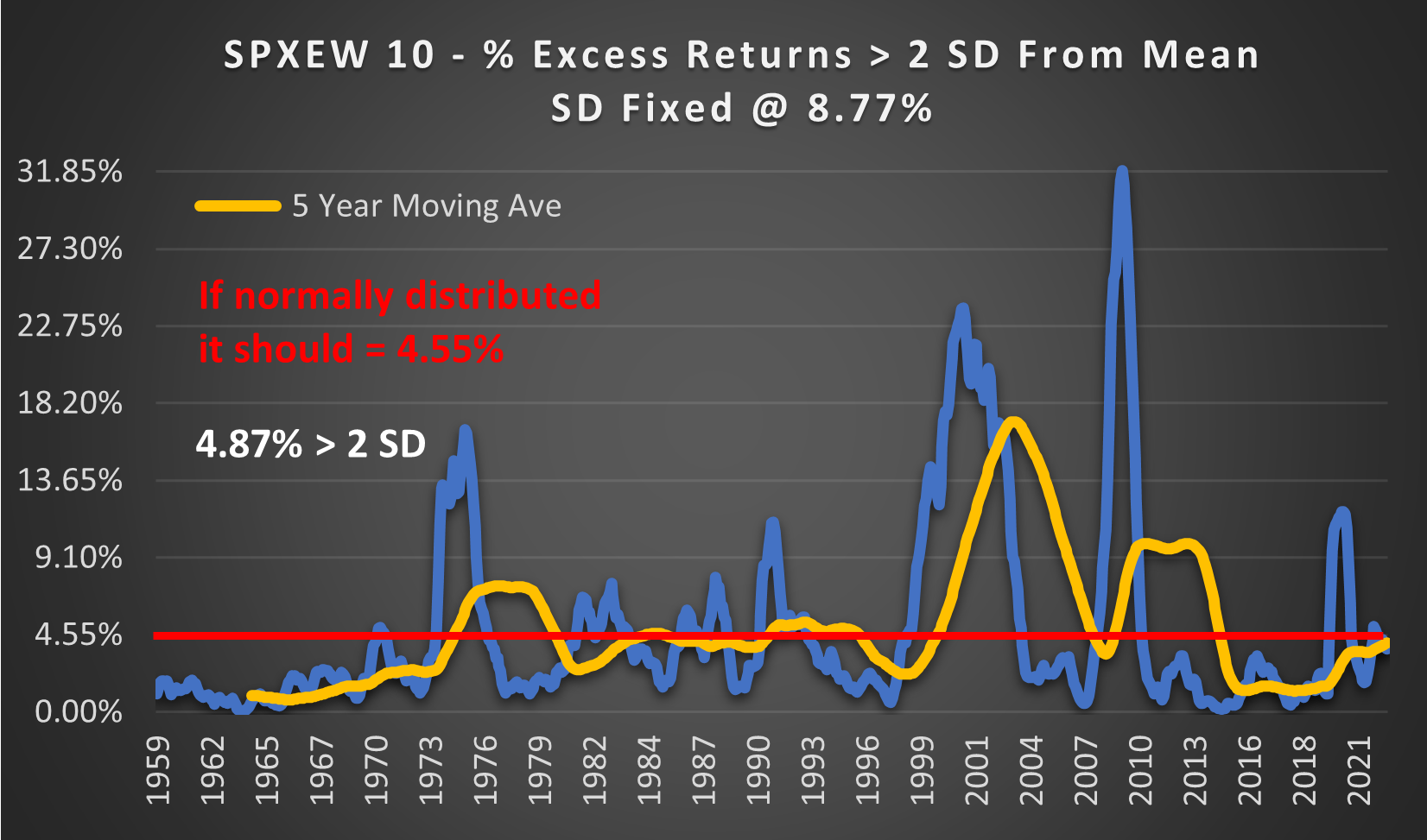
(Above) Here you can see the very obvious fat tails. In 2009 over 32% of outcomes were 3.65 Standard Deviations from the mean. This should only happen once in every 3846 years. Surprisingly, overall only 4.87% of outcomes are > 2 SD vs 4.55% for a normal distribution. Much less than I was expecting.
Instead of using a fixed Standard Deviation taken from the entire range, what if we used a rolling Standard Deviation taken from the previous year? If last year’s SD had any predictive insights into next year’s SD then we would expect the outcomes > 2 SD to be more tightly grouped around 4.55%.
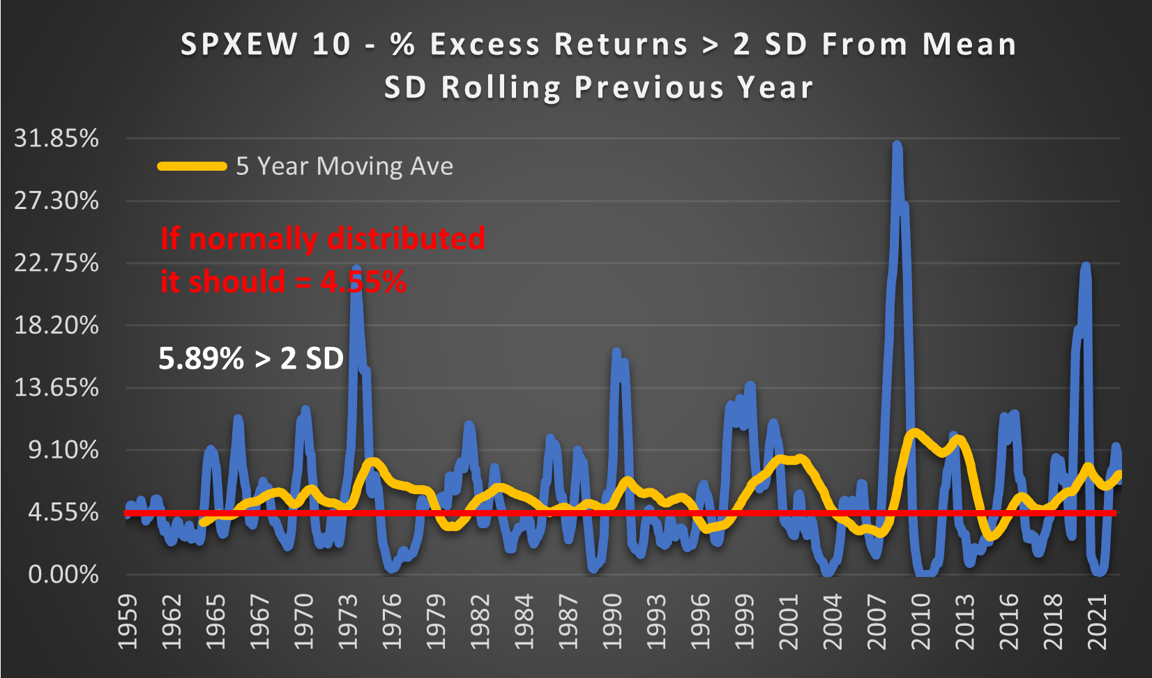
(Above) Unfortunately, we see the opposite. The percentage of outcomes > 2 SD has now jumped from 4.87% to 5.87%. Although, it is worth noting that the extreme values are similar. So it can be said that the SD this year provides no insights into the SD next year.
What if we used the SD from the current year? If the SD is known (through the benefit of hindsight) and the outcomes are normally distributed then we should see a tight cluster around 4.55%.
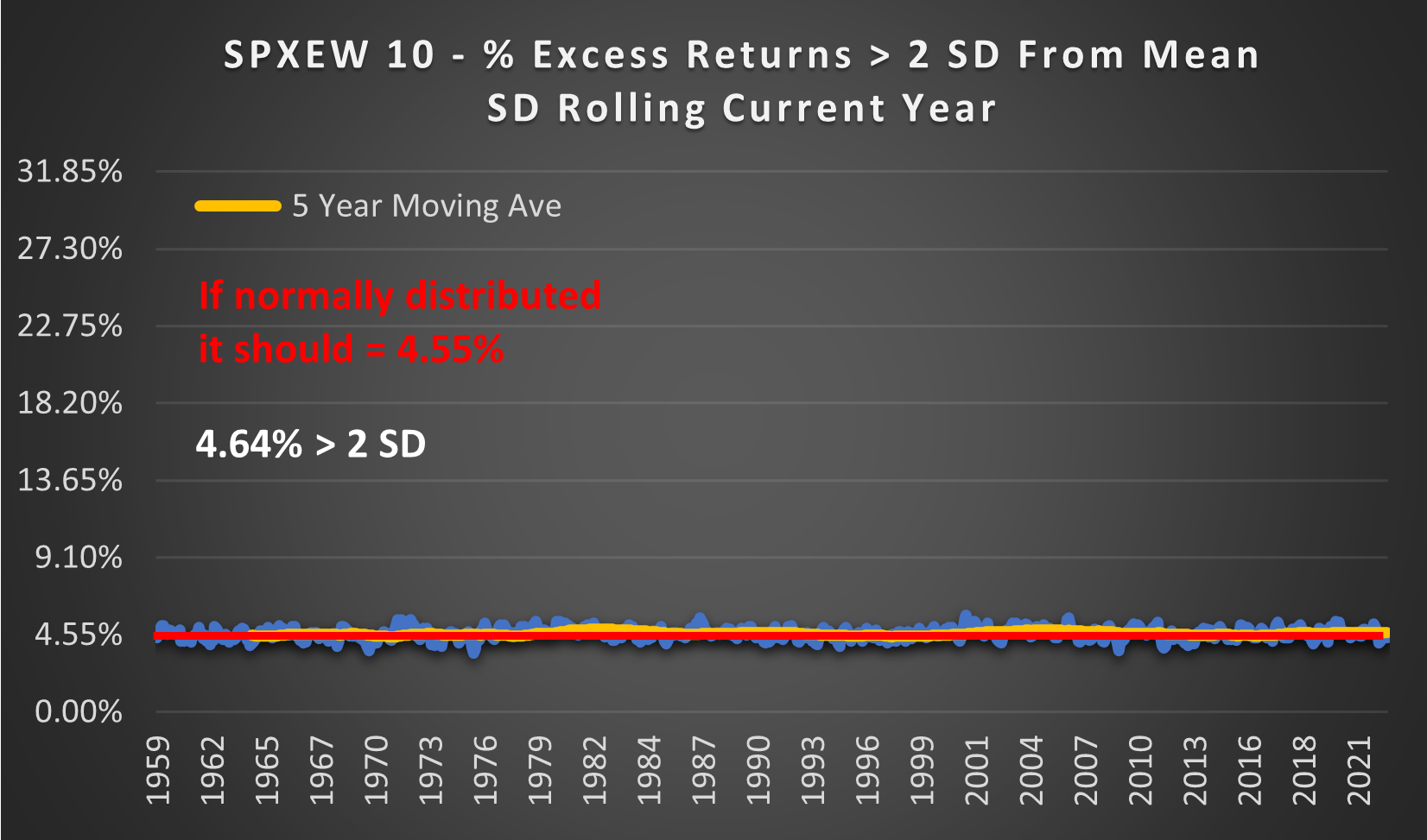
(above) And that is exactly what we see. Stock movements within a year look normally distributed if the SD is known. The trouble is we can never know what the SD will be ahead of time. The range from the highest SD year to the lowest SD year (so far) is 6.61% (1964) to 16.49% (2009). The SD for the entire history (8.77%) simply doesn’t represent the probable outcomes across such a large range so its usefulness is questionable.
Yet Standard Deviation is widely used in financial models and risk metrics such as:
Black-Scholes Options Pricing Model
Modern Portfolio Theory
Value at Risk (VaR)
Sharpe Ratio
GARCH Models
Monte Carlo Simulations
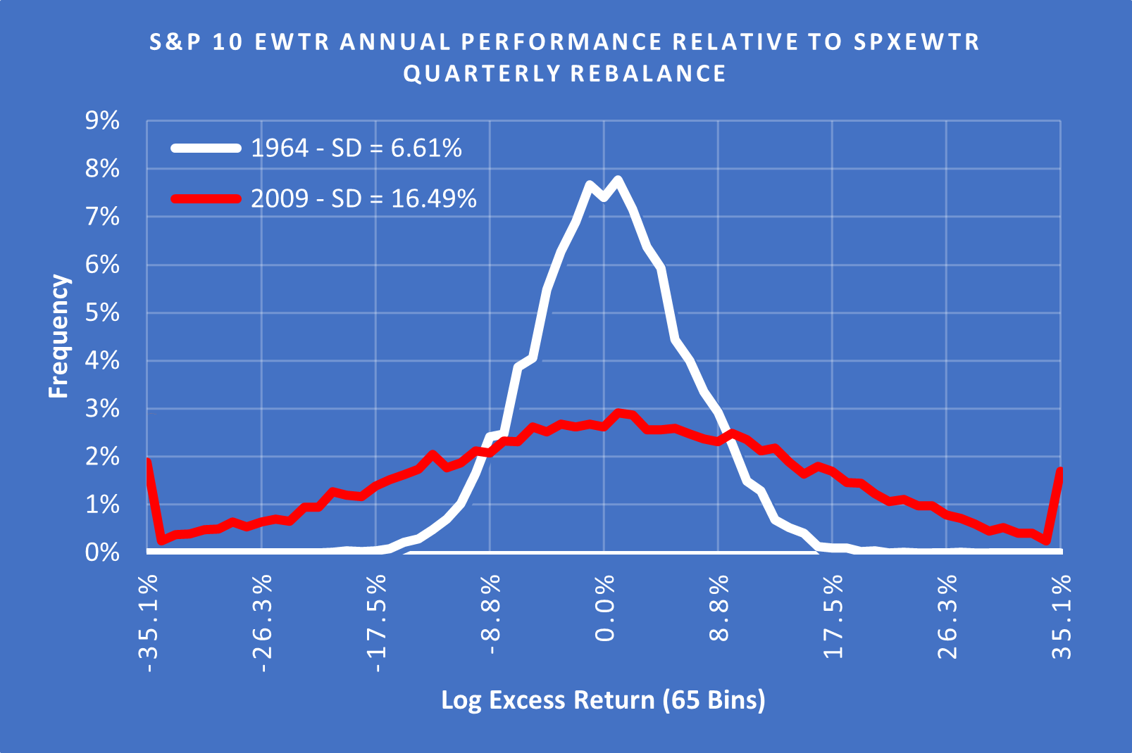
(Above) Here you can see the years with the highest and the lowest SD laid on the same scale with each point on the X axis representing one SD based on the entire 1957 - 2023 data sample. 1964 appears extremely peaked with no tails while 2009 has 1 / 25 (4%) of outcomes > 4 SD from the mean. A 4 Sigma event should only occur once every 15,787 years in a normal distribution.
However, if we look at the distribution of outcomes for each of these years using their own Standard Deviations then the data models much more cleanly.
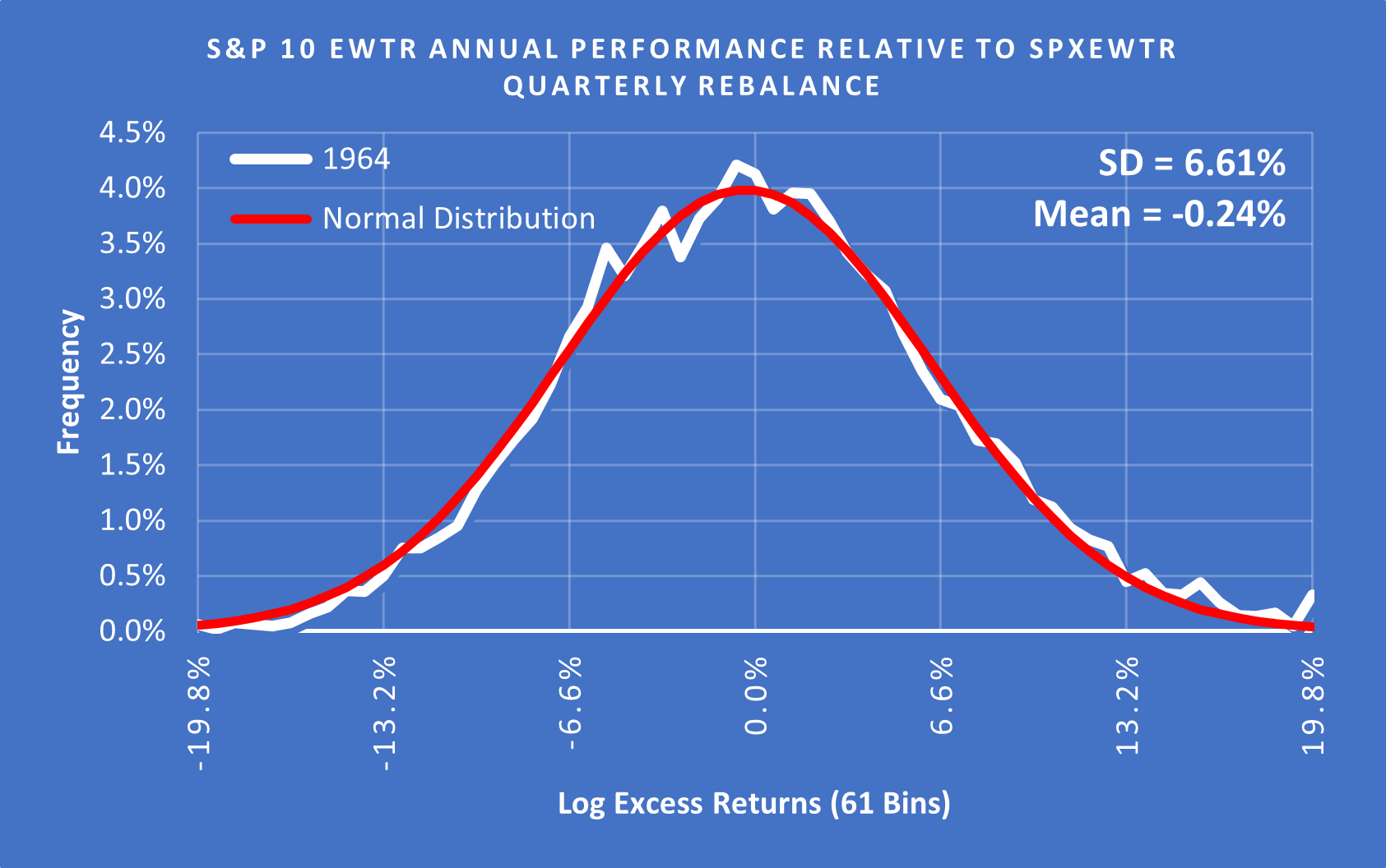
(Above) Using a SD of 6.61% for 1964 the data looks fairly normal but with a slight fat tail to the upside.
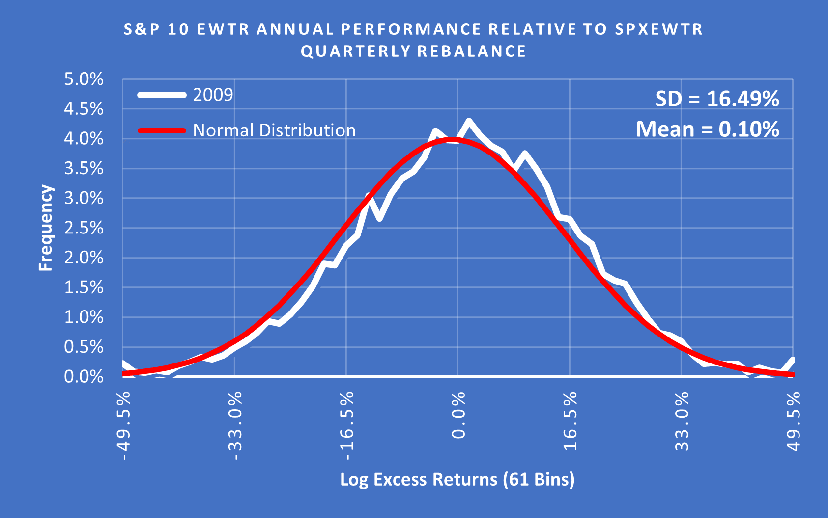
(Above) Using a SD of 16.49% for 2009 the fat tails are now quite small and while you wouldn’t describe it as normally distributed, it isn’t a terrible fit.
How does Standard Deviation Change with the # of Stocks In A Portfolio?
So far we have only looked at the distribution of outcomes for portfolios with 10 stocks. But do the numbers vary as the number of stocks change?
I found an astonishing continuity in the readings as the number of stocks changed. For 10 stocks the SD was 8.77% and for 100 it was 2.71%. However, 4.87% and 4.88% of outcomes respectively were > 2 SD from the mean. So while the SD was very different, the distribution remained the same.
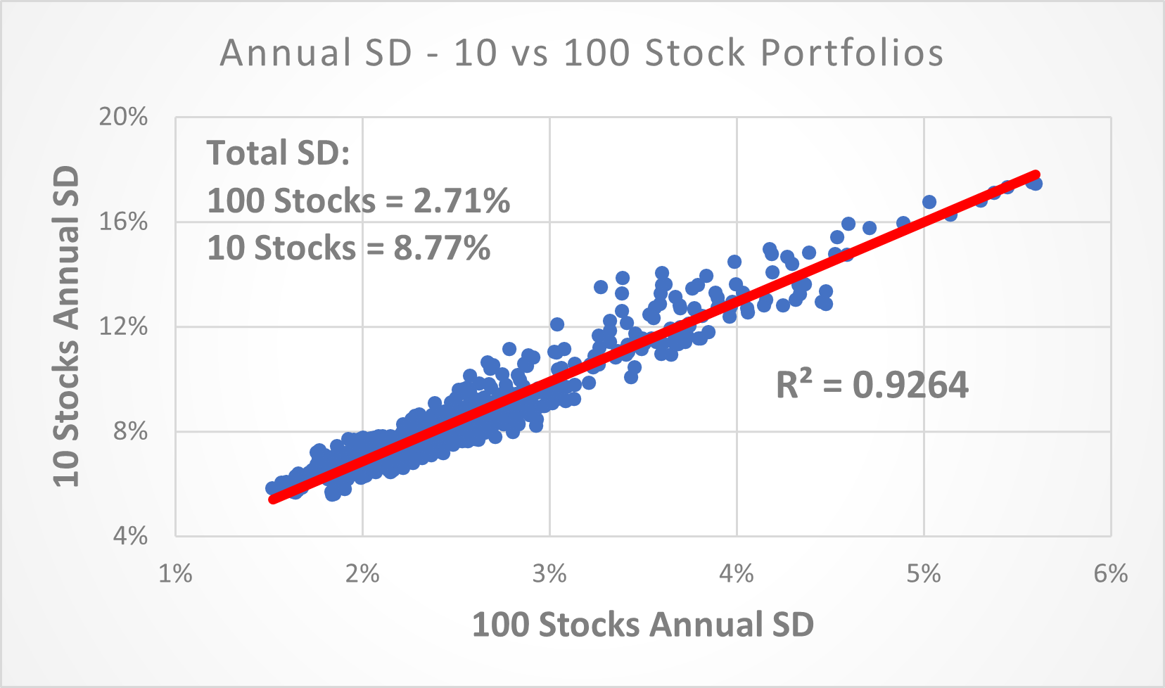
(Above) The R² for the Annual SD between the 10 stock vs. 100 stock portfolios was 0.9264. Meaning that ~92.64% of the annual variability in the SD of the 10-stock portfolios can be explained by the variability in the SD of the 100-stock portfolios. The actual R² is likely even higher since I only ran 100 simulations for the 100-stock portfolios vs 1,000 for the 10-stock portfolios.
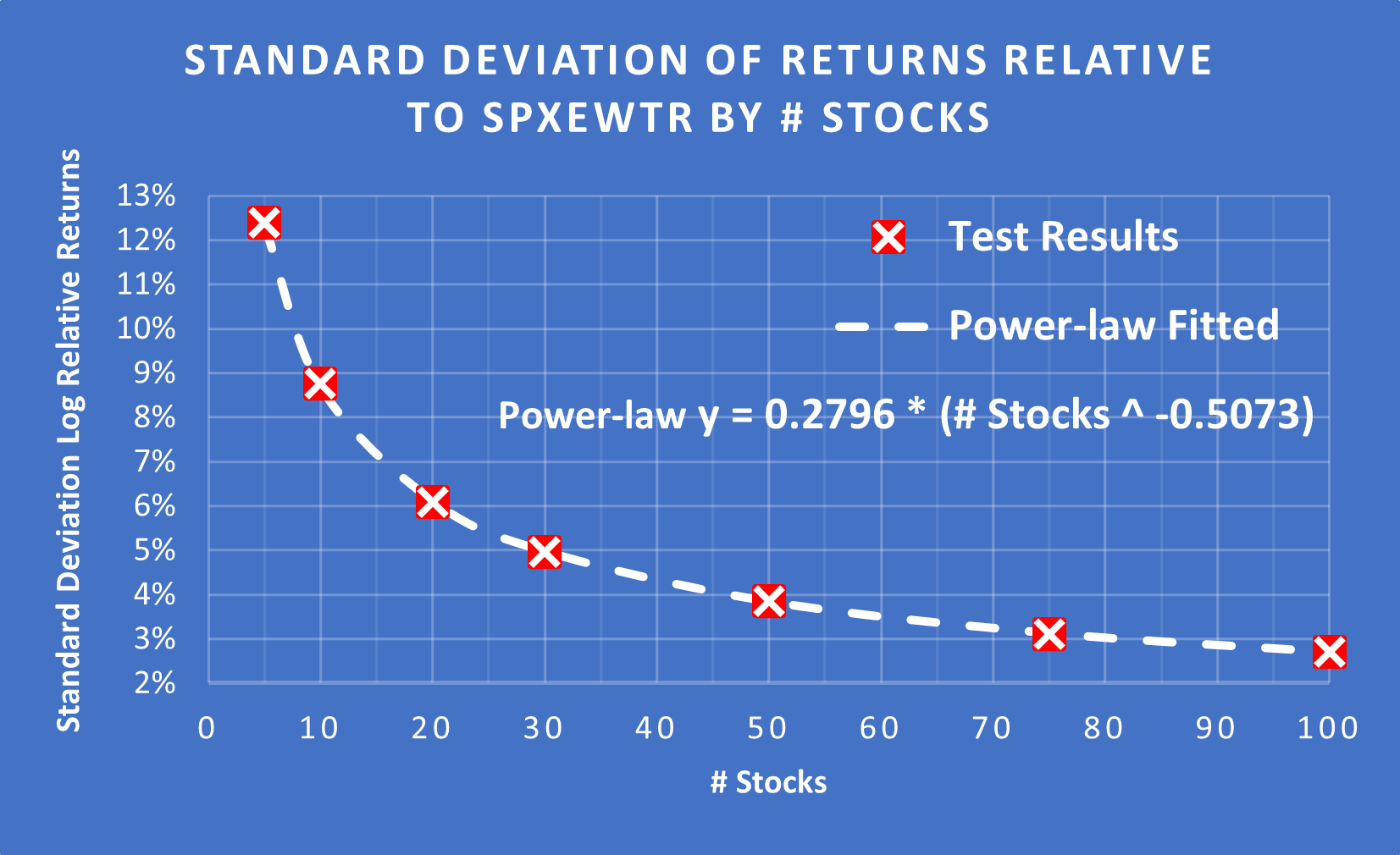
(Above) The change in the Standard Deviation of excess returns is easily found as a function of the number of stocks in the portfolio = 0.2796 * (# Stocks ^ -0.5073). This curve is an almost perfect match. It is also interesting to see that most of the reduction in SD has occurred by the time you reach 30 stocks.
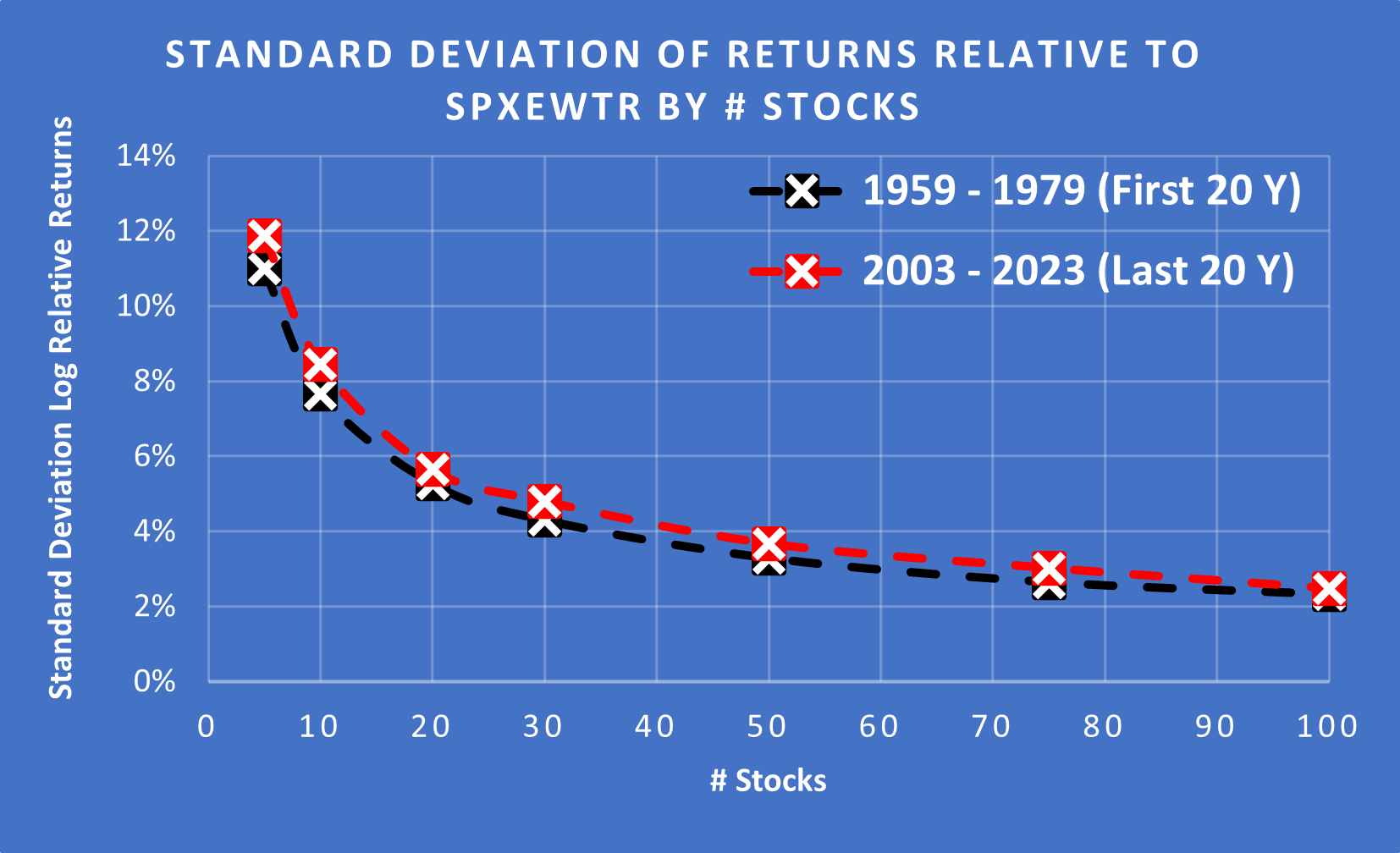
(Above) I have plotted the Standard Deviation for the first 20 years and the last 20 years. As you can see, the long-term SD has stayed remarkably stable.
Rebalance Frequency Has Little-To-No Impact
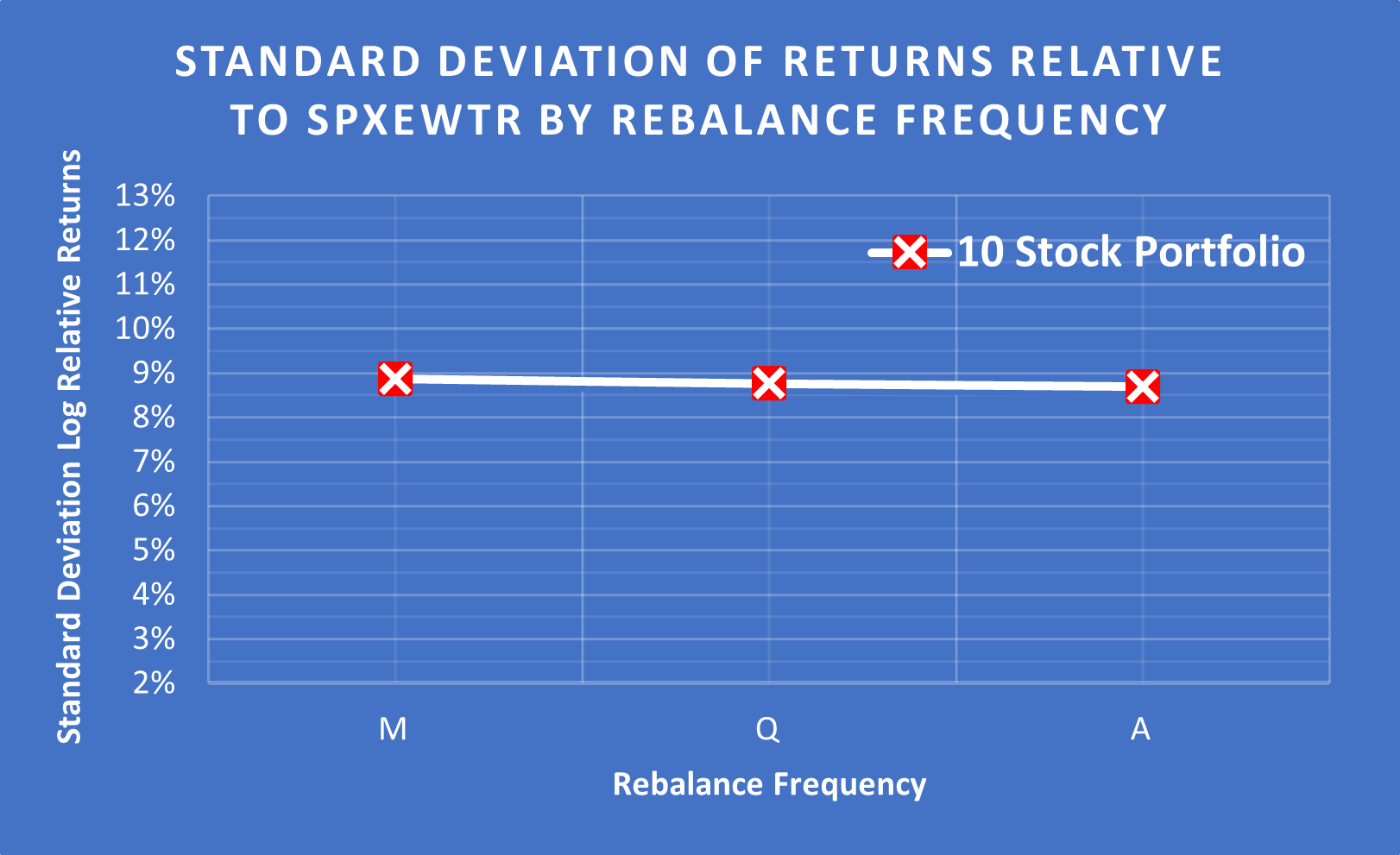
(Above) Surprisingly, changing the rebalance frequency had little to no effect on the Standard Deviation. Monthly (M), Quarterly (Q) or Annually (A).
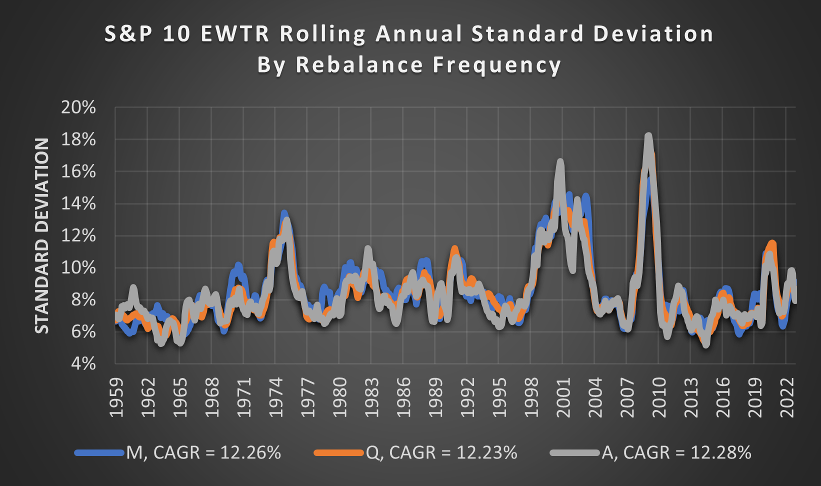
(Above) Even the Rolling Annual Standard Deviation is very similar regardless of the rebalance frequency. Astonishingly, the average CAGR is also only separated by a rounding error @ M = 12.26%, Q = 12.23% and A = 12.28%.
Obviously, a portfolio that trades less frequently will incur less trading friction and this hasn’t been factored. However, I assumed that trading less frequently would result in a higher SD because some stocks will have extreme outcomes so some random simulations will be stuck with them for an entire year instead of just one month or quarter.
How Does The Sharpe Ratio Change with the # of Stocks In A Portfolio?
The Sharpe Ratio measures risk-adjusted return. It quantifies the excess return earned per unit of risk taken, with risk represented by the Standard Deviation of returns in excess of the risk-free rate (interest on the three-month U.S. Treasury bill). A higher Sharpe Ratio indicates better risk-adjusted performance, suggesting that the investment generated more return for the amount of risk incurred.
Excess Sharpe is the Sharpe Ratio for the test results minus the Sharpe Ratio for the SPXEWTR (Benchmark).
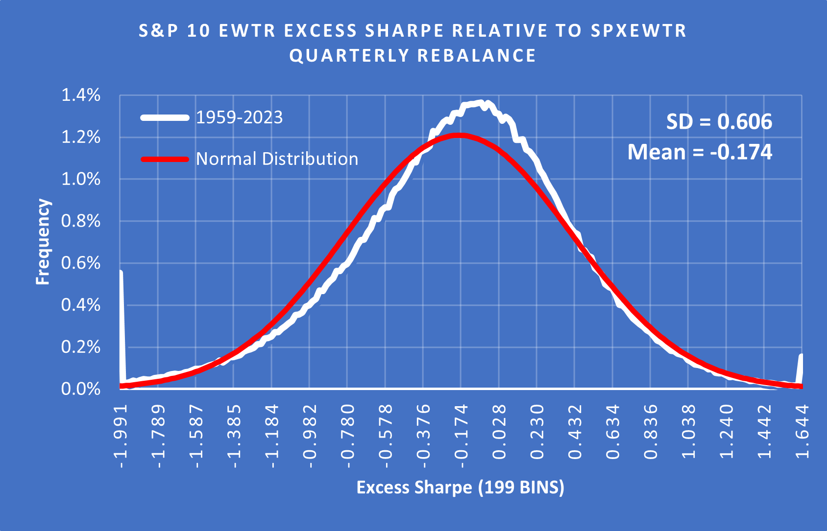
(Above) When we look at the Excess Sharpe distribution, the fat tail on the upside becomes smaller while the fat tail on the downside gets bigger. This is because extreme outcomes come with a lot of additional volatility and risk. It is interesting to see a positive skew, although the mean is below zero.
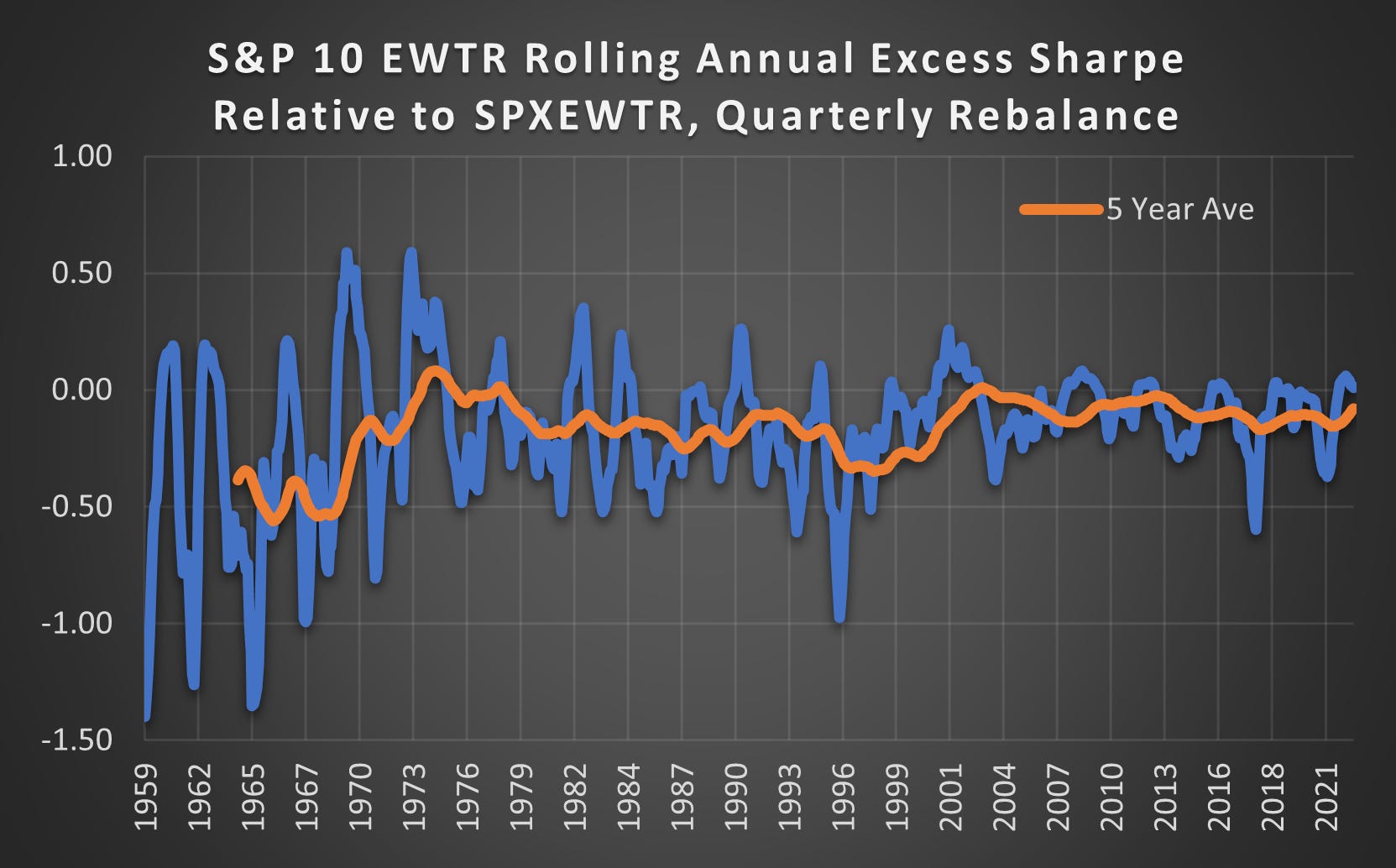
(Above) In the 60s, the negative Excess Sharpe was significant while more recently it has been close to zero. More research is required to identify what has caused this improvement. One aspect is likely to be an improvement in liquidity and an increase in correlation. If stocks are more correlated then the benefits of diversification can be achieved with fewer stocks.
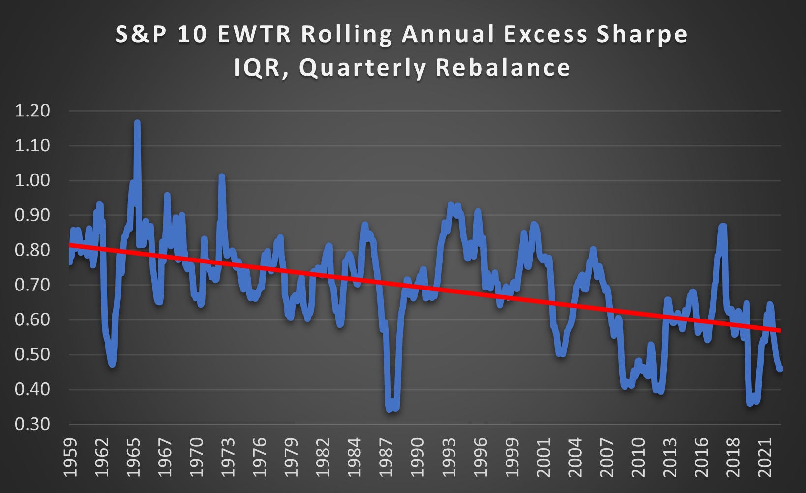
(Above) This is the Inter Quartile Range (IQR) between the Upper and Lower Quartile for the Rolling Annual Excess Sharpe. The range has declined by ~25% showing that the spread of outcomes had declined and not just the average.
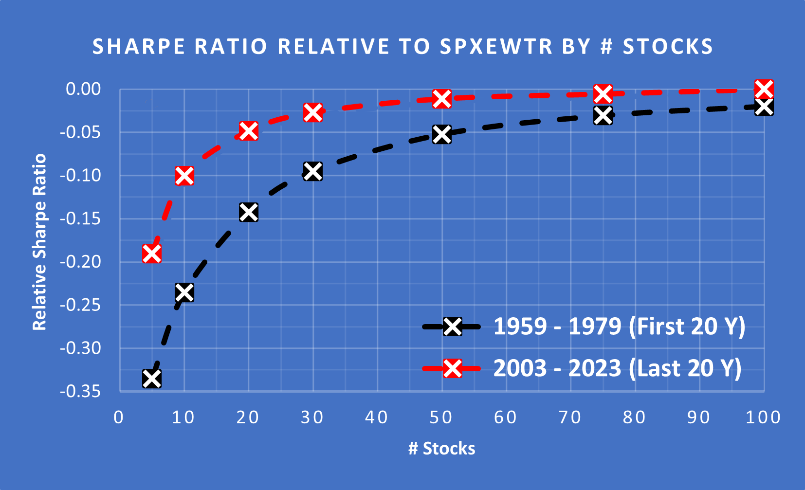
(Above) Earlier in this article we looked at how the Standard Deviation during the first 20 years and the last 20 years had remained very consistent. In contrast, the Excess Sharpe has improved dramatically. Today, you get the same risk-adjusted returns from a portfolio of 30 stocks (from the S&P 500 picked at random) as you did from ~85 stocks in the 60s and 70s.
In fact, with 30 stocks, the Excess Sharpe is only slightly negative so you have almost the same risk-adjusted returns as holding the entire S&P 500 EWTR.
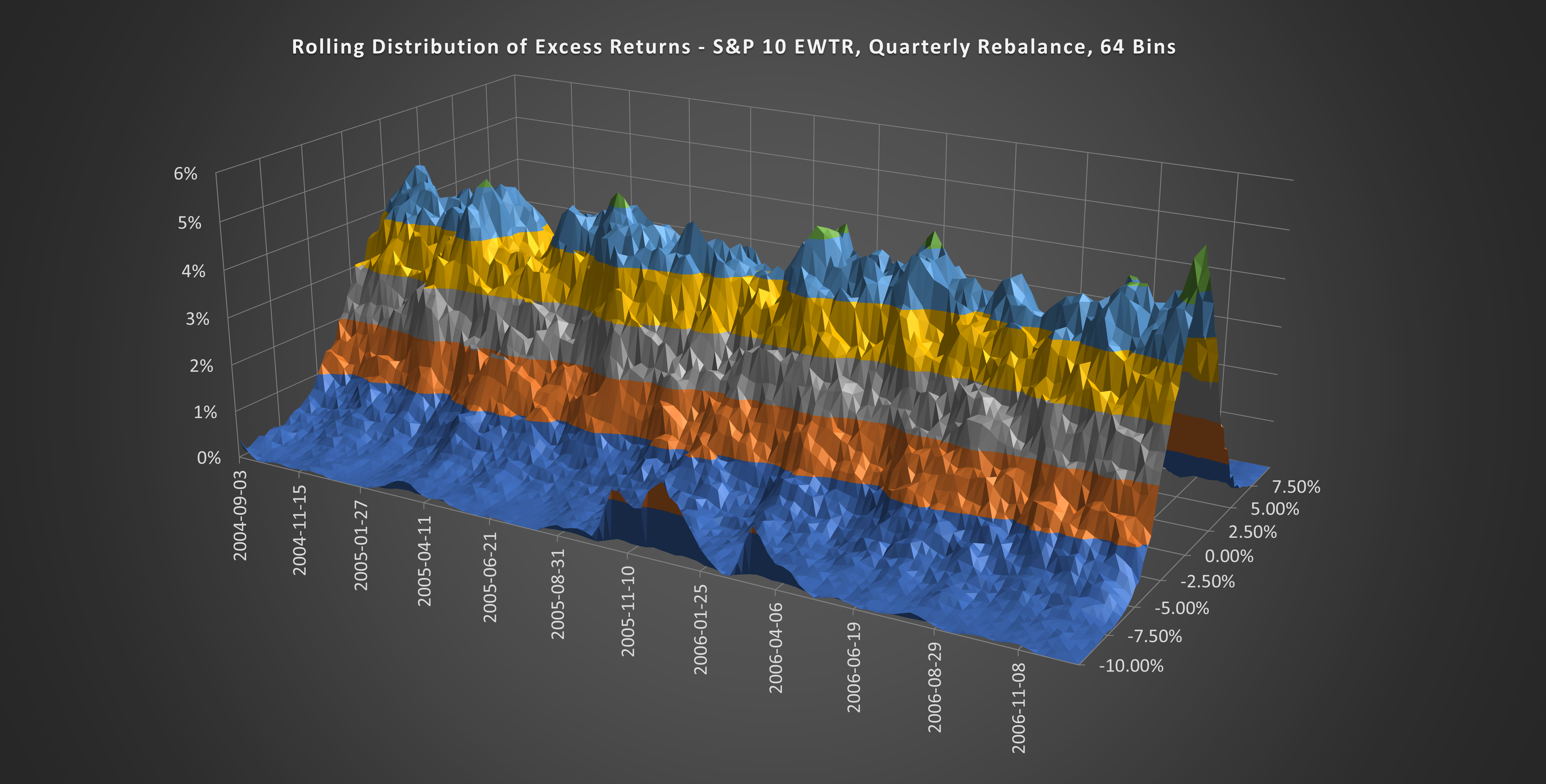
Distribution of Excess Returns Through Time

(Above) What we are looking at is the Annual Rolling Distribution of Excess Returns. Each data point on the X-Axis moves forward one-quarter. The SD is fixed @ 8.77% and the Z-Axis covers 4 SD from the mean.
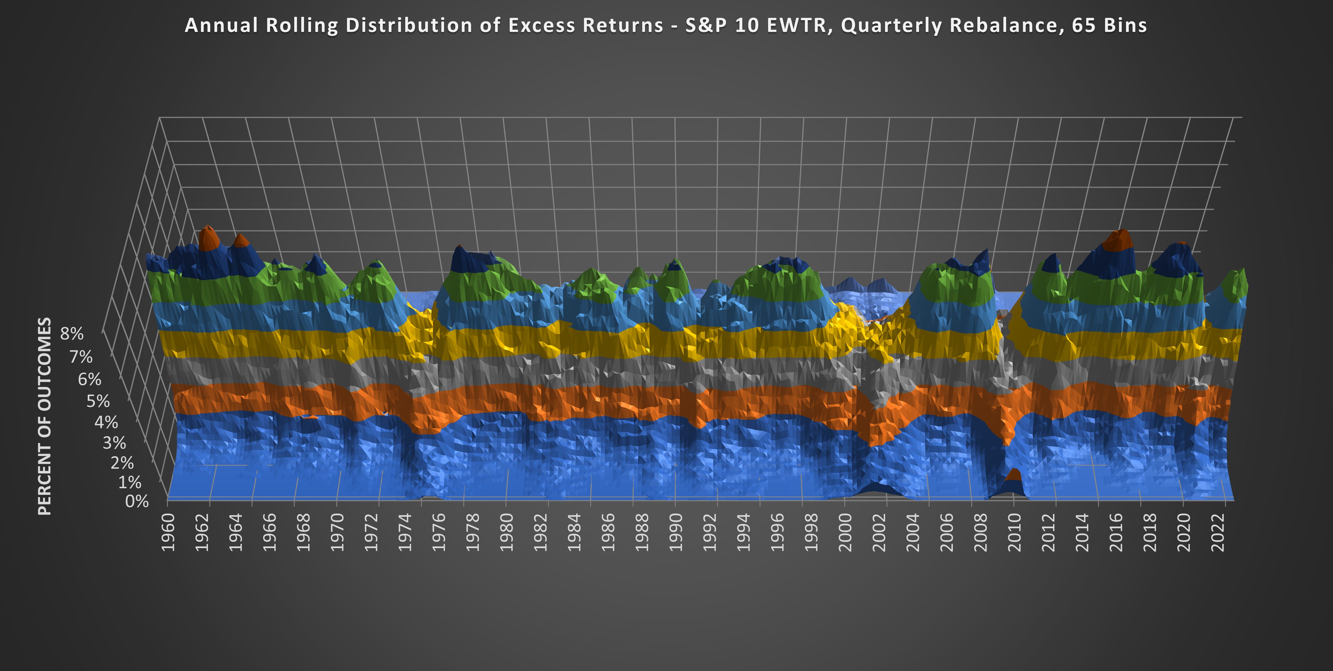
(Above) Here is the same chart from a different angle. Those who know their stock market history will notice that the distribution peak collapses during market declines and fat tails emerge.
Distributions Collapse Prior to A Crash
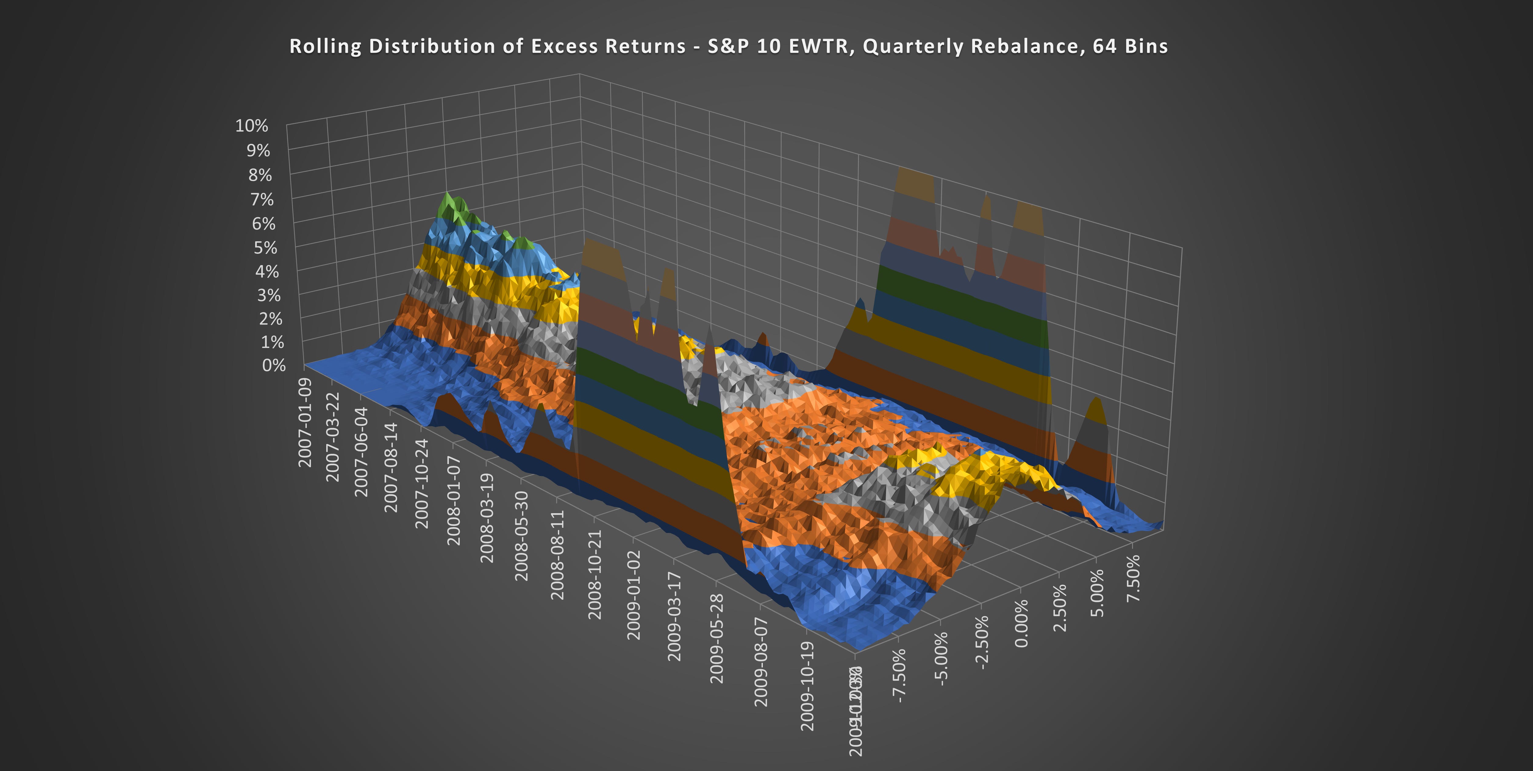
(Above) His is a more granular look at the outcome distributions, this time with weekly increments. The period pictured is the lead-up to and aftermath of the Global Financial Crisis (GFC). Notice how the distribution peak fell in the last quarter of 2007.
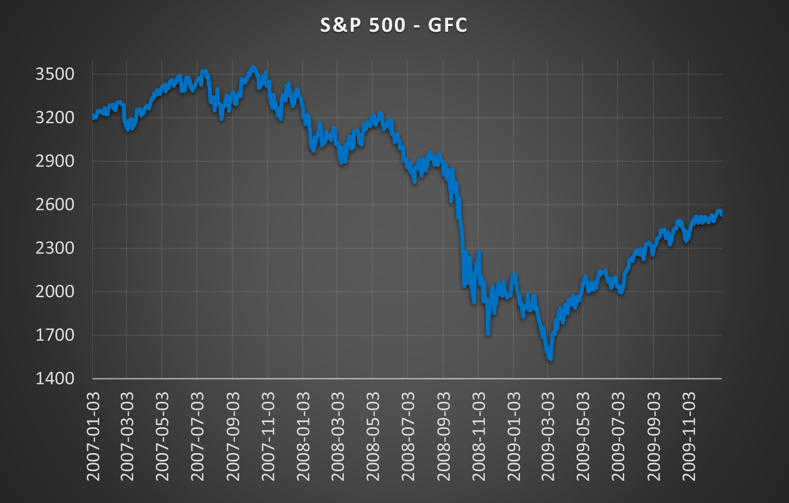
(Above) Here is the price action during the same period. The market crash didn’t occur until September 2008 but the broken distribution was warning of extreme turmoil in late 2007.
(Above) Compare the collapsed peak in 2008 to this nicely peaked distribution during the credit boom 2005-2006 for an example of a healthy vs unhealthy market.
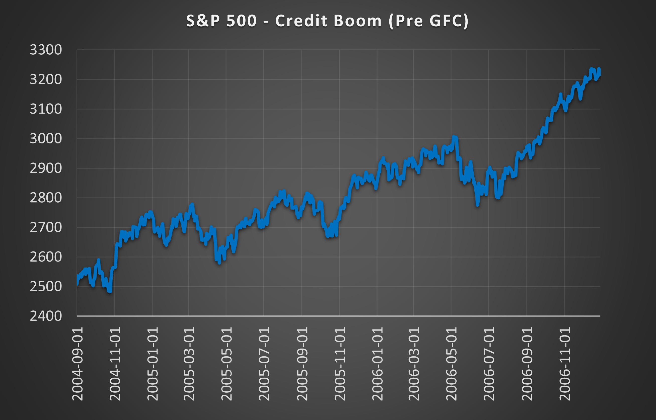
(Above) Here is the S&P 500 during the same expansionary period leading up to the GFC. Despite several pullbacks, none of them resulted in a collapsed distribution.
Conclusion
I started this research with the innocent question “How much of a portfolio’s annual performance can be attributed to good or bad luck?” I didn’t foresee how deep I would fall down this rabbit hole. It has been a few months now.
Answer: Over 20 years, 14 of those years you can expect a 10-stock, US large-cap portfolio to move +/- 8.77% relative to the S&P 500 Equal Weight Index (before trading costs) purely through luck. 5 years are likely to be +/- 8.77 to 17.7%, and 1 year +/- 26.3% or more.
Findings (True of US Large Caps):
The Standard Deviation of annual excess returns remains stable @ ~8.77% when you are looking at periods > 20 years (Long Term).
The (Long Term) Standard Deviation of excess returns is a function of the # of stocks in a portfolio = 0.2796 * (# Stocks ^ -0.5073).
Year-to-year excess returns are poorly described using a long-term standard deviation. Long periods of peaked distributions are punctuated by unpredictable fat tails.
The standard deviation for any given year (short-term) nicely describes the excess returns for that year. But the standard deviation can’t be known ahead of time.
The range of Annual Standard Deviation for Excess Returns for SPXEW 10 (so far) is 6.61% (1964) to 16.49% (2009).
Rebalance frequency (excluding trading costs) doesn’t impact the Standard Deviation of excess returns.
The relative shape ratio has declined significantly over time. You get the same risk-adjusted returns today (2024) with ~30 stocks as you used to get with ~85 stocks in the 1960s.
A distribution collapse precedes long-term bear markets.
Further Research
In my next article, I will publish more details on how outcome distributions can be used to manage risk and as an input for trading models.

NOTES
Parameters:
Universe = Active holdings of the S&P 500, 1957 - 2023 excluding any stocks that had been in the index for less than 1 year.
Benchmark = S&P 500 Equal Weight Total Return SPXEWTR (This includes dividends).
Stock Data = Price adjusted for splits and dividends.
Rebalance Frequency = Stocks randomly selected Monthly (M), Quarterly (Q) or Annually (A).
Fees and Slippage = No.
Log Returns = Yes, unless otherwise stated.
Glossary of Terms:
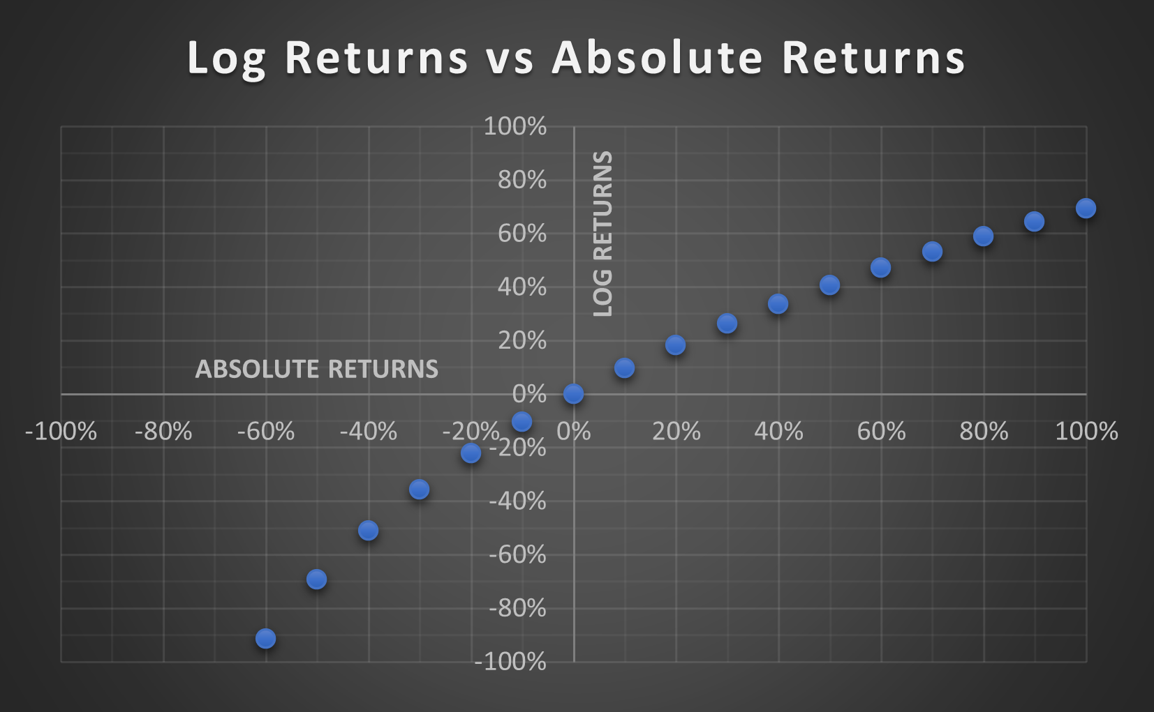
Log Returns:
If your portfolio is down by 50% one year and up by 50% the next, what is the value of your portfolio? Your brain wants to say it is back where it started but in reality it is down by 25%. You see, a 50% loss requires a 100% gain to recover. Buy using Log returns, positive and negative outcomes are adjusted so they require the same return to cancel each other out:
Log 0.5 (50% loss) = -0.69315
Log 2.0 (100% gain) = 0.69315
This allows us to fairly represent positive and negative returns proportionally on the same scale.
Bins:
These are predefined intervals used to group data points. On many of the charts through this article, you will see the number of bins specified. This means that the X or Z axis has been split into X number of “Bins” and the readings show how frequently outcomes occurred within the range of each “Bin”. E.g if there is a range of 100 with 5 Bins then each Bin covers a range of 20 and shows how often outcomes occurred in that range.
This method of data organization helps to visualize the distribution of values, making it easier to identify patterns.
Excess Returns and Excess Sharpe:
This refers to the over / under performance of a test relative to the benchmark. So if the benchmark went up by 2% and the test went up by 3% then the excess would be 1%. If the test only went up by 1% then the excess would be -1%.
Additional Point of Interest:
Alternative Method for Estimating The Standard Deviation Of Excess Returns
I noticed that the Inter Quartile Range (IQR) for the 252-day Historical Volatility of all holdings in the S&P 500 matches very closely to the Annual SD:
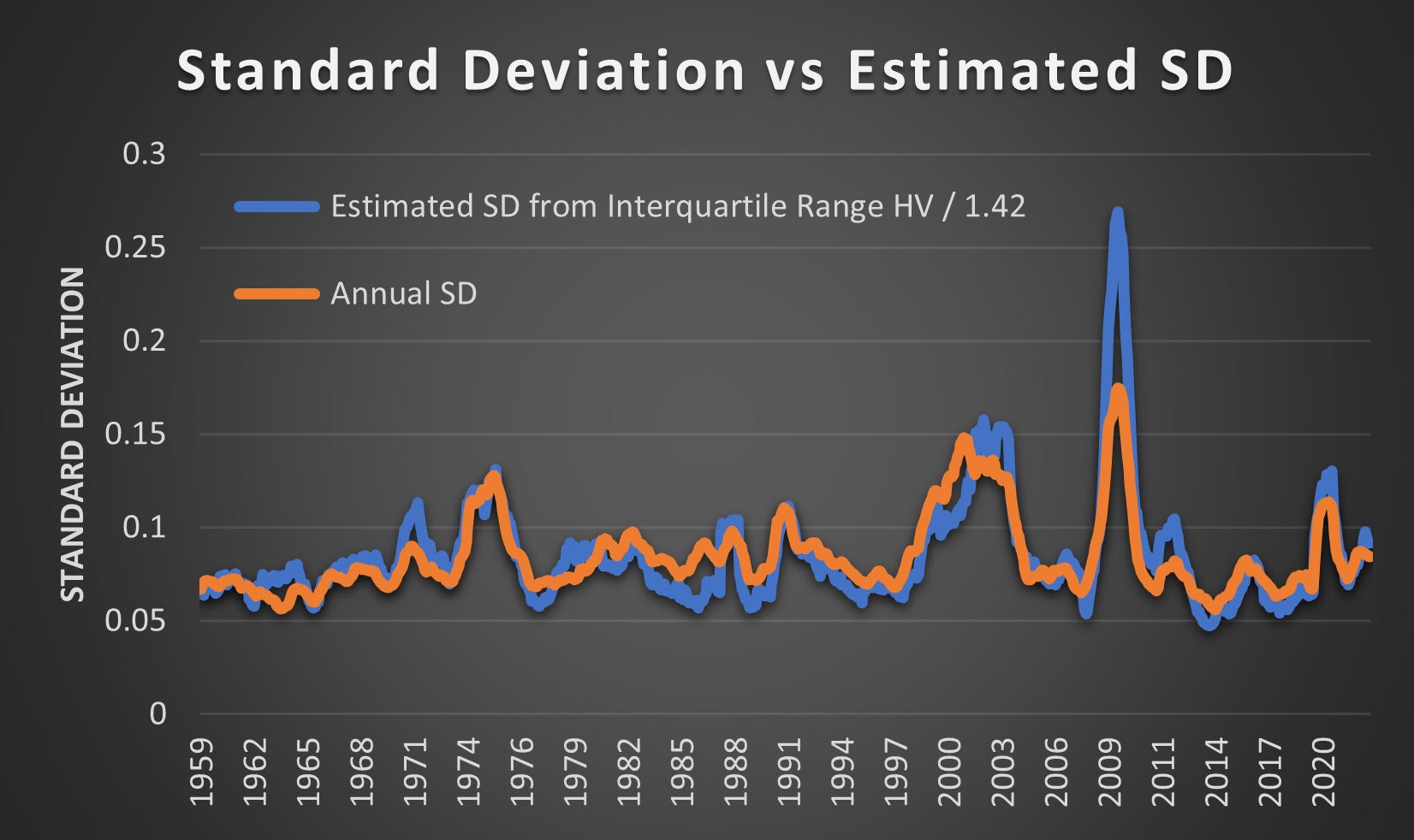
(Above) Dividing the IQR of the Annual Historical Volatility IQR by 1.42 results in a fairly tight match. It was only in 2009 that the estimated SD significantly overshot.
The required ratio for the conversion can be calculated based on the number of stocks in the portfolio:
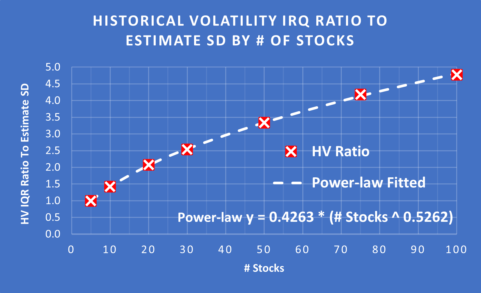
(Above) The required ratio = 0.4263 * (# Stocks ^ 0.5262)
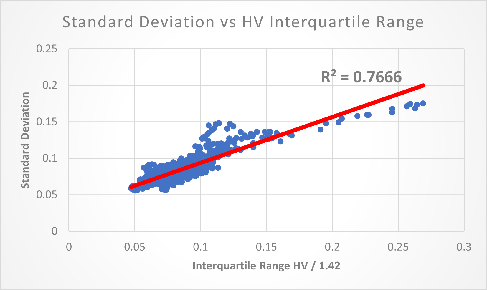
(Above) 76.66% of the Standard Deviation can be explained by the IQR of Historical Volatility.